Gordon Lichtstein
A website for my code, projects, and bio
Graphing the English Language: A Network Theory Approach to Synonym Mapping
A project analyzing English with synonyms, NLP, and network theory by Akarsh Duddu and Gordon Lichtstein.
Code and data can be found at https://github.com/generic-account/syn_mapping.
Introduction
What does a language look like? And what does that question even mean?
Well I had this very thought a few days ago, and while ordinarily I might dismiss it, I decided to pursue my curiosity. This led me down a path through natural language processing, massive datasets, high-performance computing, network theory, and graphical visualization tools.
The core of this project is to map the semantic content of words and language - what it means. But the meaning of words don’t truly lie within them or the letters that make them up, but instead by the words that are similar to them in meaning, appear in similar contexts, and have similar relationships to other words (e.g. two words sharing synonyms, even if they aren’t synonyms themselves).
Libraries and Software Used
This project is primarily done in Python, and I will be using the following libraries throughout this project: NLTK, Networkx, and Matplotlib. Although Python isn’t the fastest language (and we will run into some difficulties with it later on), it is sufficient for much of the project.
NLTK, or the natural language toolkit, provides numerous NLP (natural language processing) tools, but we will primarily be using its implementation of Wordnet (https://wordnet.princeton.edu/), which is an English lexical database of “sets of cognitive synonyms (synsets), each representing a distinct concept.”
Networkx is a graph library for Python supporting the “creation, manipulation, and study of the structure, dynamics, and functions of complex networks”. I largely use it to easily create and export graphs with Python, as it is too slow for many more computationally intensive tasks.
Matplotlib is a library that’s incredibly useful at making statistical visualizations in Python, including histograms, graphs (like the ones I make here), scatter plots, and multivariate visualizations. I used it for the first parts of this project, but it scales poorly as my dataset size increases.
Other than the Python libraries, I will also be using Gephi which is a network visualization and science tool. It will be the primary tool I use after generating my datasets in Python, as it’s very fast and easily supports multi-processing in some scenarios.
Dogs and Recursion
My initial thought was to do this recursively - take some word and add all its synonyms. Then take all those synonyms and add their synonyms. Then take those synonyms of synonyms and add their synonyms, and so on until we have added every word and its synonyms. So I implemented this. And what better word to use than “dog” (don’t say “cat”)?
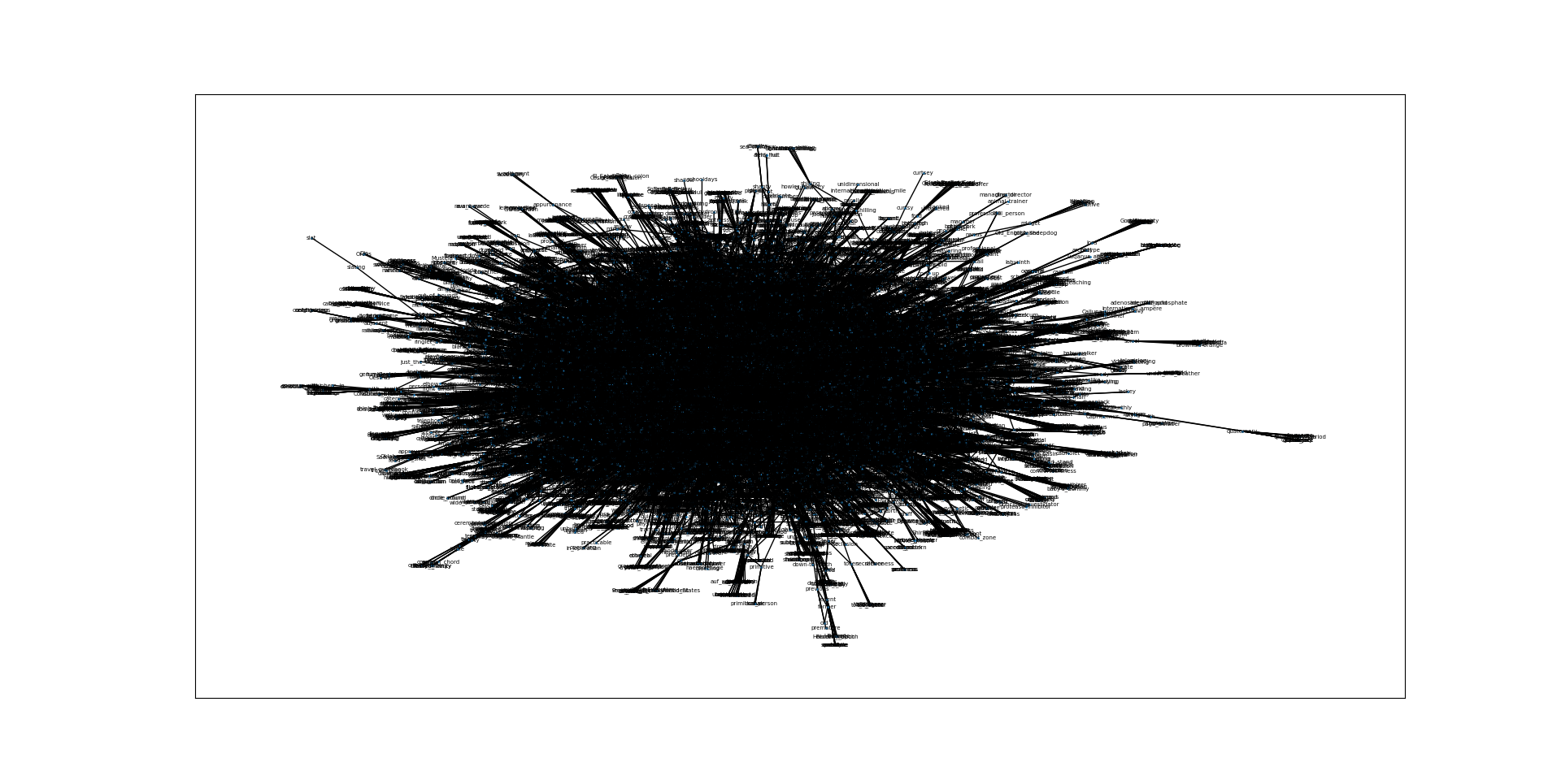
Of course, I couldn’t go all the way at first, so I wrote a function that adds nodes and edges to the Networkx graph recursively up to a certain depth. The results of the depth = 5 graph is below. In matplotlib this is interactive, so you can scroll around and zoom in to view things more clearly. However, its visualization features are a bit lacking, and even visualizing this was very slow, which should have been a bad sign for the rest of this project.
First, I have a basic driver class that manages some of the graph edge addition and visualization parts. See code below.
class Graph:
    def __init__(self):
        self.lst = []
    def addEdge(self, a, b):
        self.lst.append([a,b])
    def visualize(self):
        G = nx.Graph()
        G.add_edges_from(self.lst)
        nx.draw_networkx(G,font_size=5,node_size=1)
        plt.show()
I have a function that takes a word and gets all of its synonyms. This works by getting the synsets of a word (a list of lists of connected synonyms), and flattening it into one list of synonyms. See function below.
def get_syns(word):
    synnets = wn.synonyms(word)
    final = []
    for i in synnets:
        for j in i:
            final.append(j)
    return final
Then, very simply I have a recursive function that takes one word and a depth as arguments. It retrieves the synonyms of the word, adds that synonym link, and then passes that word in an argument to itself recursively (with the depth decreased). This will terminate once the depth is equal to zero, so we don’t continue running forever.
def add_syns(word,depth):
    if depth == 0:
        return 0
    syns = get_syns(word)
    for syn in syns:
        G.addEdge(word,syn)
        add_syns(syn,depth-1)
This works, but there are a few problems with this approach. One is that if two recursive branches somehow end up on the same word, we will end up repeating a lot of computer time. Another problem is that we are not guaranteed or likely to reach every word. English language synonyms might not be a fully connected graph, and in fact we would expect it to not be connected. If it were, this would imply that every word is a synonym of every other word, which obviously is not true. But because of this lack of connectedness, the recursive algorithm will get “stuck”. It will only be able to visit the neighborhood of points that care connected to the word I initially put in (in this case “dog”). This approach is slow and incomplete, so what’s better?
Sequential Approach (and Scaling)
My next approach was a sequential one, where I would go through the words in some word list, and add each of their synonyms to the graph. Much of the code was very similar, except for the bit that interacted with the word list and the way I loaded the graph.
I found two wordlists that seemed good to test on. One was the top 10,000 most common English words, and the other was about 400,000 words. I figured the 10k word list would be a good test, and I could always increase the number of words.
Because of the sheer volume of words, I thought that adding synonyms one by one as I did in the add_syns function above would be too slow. As such, I took advantage of another feature of the networkx library, which is loading from an adjacency dictionary. This is a dictionary where the keys are nodes, and the values are tuples of nodes that are connected to the key node. I made a function to build this adjacency dictionary (see below).
def gen_adj_dict(words):
    d = {}
    for word in words:
        d[word] = tuple(get_syns(word))
    return d
Other than that, the code was mostly the same. I opened the text file of the word list (one word per line), and went through it line by line, adding each word to a list of words. Then, I generate the adjacency dictionary with this list of words, and generate a graph based on it. Then, as networkx's draw_network function was getting too slow, I saved the graph as a .gml file (a standard graph file format) for viewing and processing with other programs. See the code below.
with open("400k_words_alpha.txt", "r") as f:
    words = [line.strip() for line in f.readlines()]
print("file read")

adj_dict = gen_adj_dict(words)
print("adj dict done")

G = nx.Graph(adj_dict)
print("graph generated")

nx.write_gml(G, "top_400k.gml")
print("graph saved")
Multiprocessing
I initially thought that the bottleneck in my code was the generation of the adjacency dictionary, and that I would have to use the Python multiprocess or multiprocessing module. This was before I switched away from using a Python visualization via draw_networkx. However, I did a bit of research and using multiprocessing seemed like a bit of a pain, so I decided to reevaluate whether or not I actually needed it. Instead of assuming, I first decided to do a bit of testing to see where the bottleneck actually was. It was a good thing I did.
After adding a few simple print statements after each line of meaningful code, I determined that adding the 400k words and their synonyms to the graph was not actually very slow, and it only took a few seconds. Instead, the bottleneck was in the visualization. This led me to saving the graph as a .gml so I could visualize it other software, such as Gephi.
While this was the end of my thoughts about multiprocessing in Python, it was not actually the last time it came up in this project. Gephi uses some algorithms that can take advantage of multiple cores, and this was key for me being able to process the 400k document in any reasonable amount of time.
Visualization with Gephi
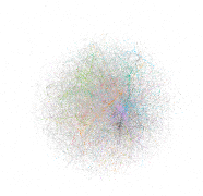
The following graph has been laid out with the OpenOrd algorithm, an efficient algorithm for making visually pleasing graphs that works particularly well with very large graphs.
Network Theory with Gephi
One can extract multiple statistics from a network to better understand it. Our aim with the synonym graph is to map and understand insights from it.
Well what are the statistics that we can extract?
Degree
The degree of the is the the number of edges, or synonym connections, a single node (word) has. We know that “take” has one of the highest degrees at 272, indicating that it is a very general word with multiple meanings in multiple contexts. For example, the word can be used to obtain a physical object (e.g, “I took a slice of pizza”) but can also be used in the context of filming with multiple “takes” needed to film a scene.
Average Degree
The average degree is the mean number of synonym connections a word has. Generally, a higher value of this statistic shows a more interconnected network. The graph has an average degree of 1.771.
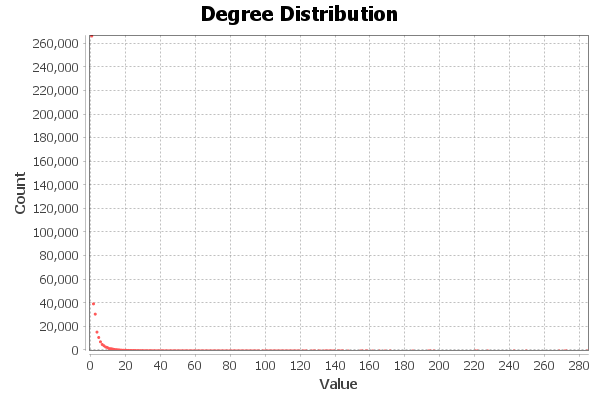
We can clearly see that the degree distribution of all the nodes in the graph is right-skewed. With a peak of 260,000 words without any synonyms, we find that a lot of the nodes in the network are isolated vertices. Despite many words on the right having a high degree, their pull on the mean of the distribution is too weak compared to the large number of words with very few synonyms.
Diameter
The diameter is the maximum possible distance between two nodes in a graph. Even in a graph with 400,000 words, it is surprising to see that the largest possible path necessary to connect two points is only 22. This tells us that the English language is much more connected in meaning than is expected.
Modularity
Modularity is the measure of the strength of groups, or communities, in the graph. Measured using the Louvain Algorithm, a higher modularity indicates a graph with large distinct clusters, likely being words with similar semantics.
We see that the modularity of the English language is 0.876, which is a considerably high value. Our data is very modular, splitting into neat chunks that are tightly interconnected amongst themselves. We can expect this, because a word’s close synonyms are synonyms with each other.
It would be interesting to see what these communities look like. Directly from Gephi, we get a graph of different modularity classes: groups of nodes determined by the algorithm to be communities in the graph. Below is the size distribution of the different communities in the graph:
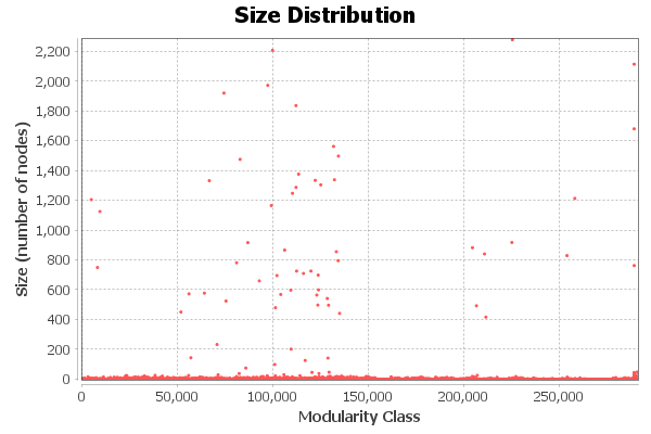
The x-axis represents each modularity class (i.e., Modularity Class 0, Modularity Class 1, etc.). We can get some interesting insights by seeing which classes are the largest, so we wrote a quick Python script to find the five largest ones:
from collections import Counter
import pandas as pd

syn_df = pd.read_csv("top_400k.csv")
NUM_CLASSES = 5

top_five = Counter(syn_df["modularity_class"]).most_common(NUM_CLASSES)

for mc, count in top_five:
    print(f"Modularity Class {mc}, Count: {count}")
Running this script, we get the following output:
Modularity Class 225099, Count: 2285
Modularity Class 99498, Count: 2214
Modularity Class 288827, Count: 2121
Modularity Class 97029, Count: 1979
Modularity Class 74076, Count: 1927
The collections.Counter class takes in an iterable of elements and counts them. Calling the most_common method with the argument of 5 gives us the top 5 highest counts. Each modularity class in this list has more than 1500+ nodes.
Average Clustering Coefficient
The average clustering coefficient is the average of each node’s local clustering coefficient. A local clustering coefficient measures the likelihood of a node’s neighbors to be neighbors themselves (forming a triangle.) The graph’s clustering coefficient is 0.654, which means on average, 65.4% of connections between a node’s neighbors are already present. This is a high value for a network, meaning the graph has many clusters and connections within clusters are very dense.
Eigenvector Centrality
The eigenvector centrality measures how influential a node is in a graph. A high value of this statistic would occur for a node that has many edges connected to it and is neighbors with other influential points.
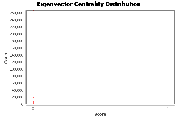
The distribution above shows that only a couple of values have a high eigenvector centrality. Upon inspecting the ‘Data Laboratory’ feature in Gephi, we come to find out that “get” has the highest value at 1.0. This does not mean that “get” is connected to every single node in the graph. Rather, it is the most influential point in the graph, and the rest of the points are standardized between nodes with no influence and the “get” node. This is similar to how z-scores are calculated in statistics, where data points are ‘normalized’ to allow comparison between graphs.
Betweenness Centrality
The betweenness centrality is similar to Eigenvector Centrality in that a node with more connections will have a higher value. However, this specifically checks how often the node falls in the path between two other nodes. In other words, a node with high betweenness centrality acts like a bridge between semantic clusters in the graph, so that nodes in one cluster need to ‘cross’ the node to form a path with nodes of another cluster. High betweenness centrality means that node is connected to many other nodes, and serves as a bridge for many paths as well - like crossroads. The highest betweenness centrality (3,663,680) is for the word “take”.
Conclusion
The English language is definitely complicated. Even with more than 400,000 words, however, we can learn some important insights from this synonym graph.
First, the English language is surprisingly connected. We might ordinarily only be able to think of a few synonyms for each word, but actually there are many. The large diameter of the graph means that semantic drift is somewhat significant. This is reinforced by the modularity classes being somewhat semantically meaningless - “Byzantine” and “meatiest” are in the same class, meaning that there are somehow denser connections between these two nodes than between nodes in other modularity classes.
It is also interesting to note that the centrality algorithms often overlapped, so despite calculating “important” nodes totally differently, they ended up agreeing on what the few most important nodes were. These nodes include “get”, “take”, “make”, and “pass”. These are all very common words in English, and it’s very interesting that these algorithms identified them as important, despite having no information about the frequency of words in text.
There is surely a lot more to learn about the English language through this data. We present some next steps and additional areas of investigation that could reveal deeper insights. Overall though, we believe this project has been very successful. It has revealed the beauty and connections with language that we otherwise might never have seen. Additionally, the project presented a great opportunity to explore and deepen our knowledge of graph theory and its (im)practical applications. It was honestly pretty fun.
Next Steps
We have major plans for digging deeper into the wonderful intersection of graph theory and language. There are still many aspects of this subject that we still have not explored, including…
- Looking at other languages
- Coloring by sentiment
- Trying more clustering algorithms and algorithms settings: By seeing the different clusters in the graph, we will understand why certain nodes have a high betweenness centrality.
- Looking at potential applications in applied NLP
- Comparing to embedding-based graphs
- Interactive graphing in the website